WP5: Simulation

This work package consists of a design derivation and simulation of the spectroscopy section of the ELT. The main goal of which is to have a holistic view of, and then to realize and optimize the simulation of the system. Essentially the aim is to show how the reduction of the bandwidth can increase the efficiency of the setup.

Files

Introduction

The first part of this work package consists of doing a rough schematic of the required components, to map down each’s relevant dependent and independent variables get an overall perspective on their relevance to one another, as well as to see how the components interact and depend on one another.

Setup

A schematic of the setup is shown below:

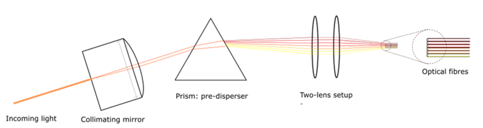
where from left to right: the limited range of incoming light first goes through a collimator which aligns the light, hence countering dispersion. Hereafter, the light can be accurately dispersed by the prism, with the shorter wavelengths at the top and the longer wavelengths at the bottom. The two-lens setup is responsible for then recollimating the dispersed light rays exiting the prism and thereafter focusing them onto the fibre optic inputs by their now separated and focused bandwidths. These highly concentrated beams can then be fed through the fibres to dispersed points to separate refined spectrometers for the finer separations. For the simulation of the part up to the fibre, we only need to simulate the side view. The top view is not required. Essentially only two dimensions (or one plane) are required at any component. However, after the fibre optic cables exit, the side view plane becomes relevant.

Figure 2 shows the top view of the setup. Here it is noted that the beam through the prism has a different dispersion to that in the side view.

Additionally, the dispersion through the two-lens setup differs between the two planes. Hence the lenses require different focal lengths for the side view and the top view.

In the top view, after the two-lens setup, six fibre optic cables are depicted schematically going into different directs to suggest that they can be directed flexibly. Note that three enlargements of the opposite ends of the fibre optic cables are shown, schematically depicting parabolic fibre couplers, each which orientate the exiting light for projection into the second dispersion layer – the high-resolution echelle spectrograph. These consist of an echelle grating which diffracts the light, separating the wavelengths onto a specialised curved mirror which then focuses diffracted waves of the same wavelength to the same points. These focused points are detected by the detectors, which interpret the incoming light.

Realistically, there would likely be far more fibre cables and associated spectrometers, which could be positioned by flexible means into many variable positions.

Components

Collimator

The collimator takes a narrow section of the bandwidth of incoming light and collimates it into parallel beams, in preparation for interaction with the prism. The collimator has two variables of main interest: the diameter of the collimating lens (d_coll) and the focal point of the collimating lens (f_coll).

Prism

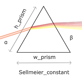
The light from the collimator enters the prism at an angle α. The light rays are then diffracted in the prism, causing the superimposed waves to split into their separate wavelengths at different angles in the prism, depending on the width of the prism (w_prism), the height of the prsim (h_prism) and the material constant (Sellmeier constant). The light then proceeds to exit at an angle β. Due to the broad-based dispersion and low losses by prisms, the prism is used for the initial low-resolution dispersion.

Two-Lens Setup

These distinguished wavelengths are then projected onto an initial lens of a two-lens setup, which acts to collimate them according to its focal length (f_lens1_side). The collimated light is then ready to be focused by a second lens with another focal length (f_lens2_side), which guides them into an array of fibre optic cables, each accounting for a specific range of wavelengths. This light is then guided through to the opposite ends of the individual fibres.

Optical fibres

The fibres have a numerical aperture (NA_fib) which is important, depending on the nature of the light. The diameter of the fibre (d_fib) and the number of fibres (no_fib) are also of relevance.

Spectrometer

Fibre couplers, at the exit end of each fibre, act to collimate the light, before it is fed into the spectrometers, each of which consists of a diffraction grating, and a camera. The spectrometers are exceptionally expensive, hence designing a system that uses an optimum amount is of paramount value.

The light is then projected into the second high-resolution spectrometer setup. Each of these several spectrometers consist of a small high-resolution echelle diffraction grating, which split the light on a fine level, a specialised lens which aligns the separated light wavelengths, and a detector which detects the light at these points.

Each spectrometer simulation should account for a bandwidth of approximately 1 nm, and a grating density of approximately 1600 - 3000 lines per mm.

CCD Detector

We only care about one dimension of the light for spectroscopy. Hence a line scan camera is used here. A CCD camera has a fixed number of pixels, which therefore is a good starting point for the simulation derivation. An initial specification of 10 pixels is decided, which can be reduced to approximately seven or eight pixels, as required.

General Degrees of Freedom

There are several degrees of freedom within the simulation, namely: the bandwidth for the small spectrograph, the number of spectrographs (more of which imply greater losses, which we don't care about), however the costs will also increase which is something that we do care about. Additionally, the system becomes more difficult to calibrate which is also of concern. Although a longer observation time may be afforded, noise and stability are the cost which are undesirable.

Parameter Optimization

To further optimize the small spectrographs an optimization algorithm was implemented,

with the goal of finding the optimal values for the different parts of the spectrograph and maximize/minimize a selectable value of the spectrograph.

This is accomplished with a gradient decent optimization algorithm.

To archive a more modular design a way to implement many different variables was designed.

Since a lot of these variables are dependent on each other and only some of them can be altered, it is possible to designate a variable either an exact value, a range of values or an equation which defines the variable.

Then one of the variables is chosen as a target to either minimize or maximize,

for which a dependency tree is built up to get the final selectable variable which the target depends on.

These final dependencies are the degrees of freedom from which we search the optimal parameters.

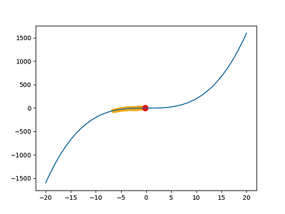
To find the desired extreme point we follow a gradient decent algorithm.

For this algorithm we start at a random point of the function and from there move our point along the gradient of the underlying function to minimize it.
We then define an exit condition at which point we are satisfied with the result of the algorithm we as well limit the iterations it can undertake as not to be stuck in an infinite loop.

The exit condition used in this code looks for a value change which is smaller then a predetermined size, if the value does not change much it indicates that the algorithm probably hit a minimum.

We also define the step size η for our algorithm, the step size has to be carefully chosen. If it is to low the algorithm may exceed its maximum iterations and not reach a minimum in time, if it is to high it
might jump between to sites of the minimum and never reach the extreme point itself.

The same process can be extended into any desirable amount of dimensions making it a good fit for this purpose.

For this use case we added edge cases to the algorithm, with each step it is checked if one of the values exceeds its allowed range, in that case the value would be set moved back to the edge of the allowed value

A problem which can arise with this algorithm is the case of a settel point. A gradient decent algorithm can have a lot of problems with saddle points as there is no gradient and the algorithm is stuck unmoving until it exceeds the maximum iterations.